Mathematics and ML

Feature Vectors Part 2

August 20, 2020

This is part 2 of feature vectors, you can continue with this without reading the part 1(Intro to vector algebra).

Analogy between Data and Vectors

In Data Science most of the times we have data in csv format. Although there are times when we have data in conventional database or other formats like json, but in most of the cases we can convert them into csv format using pandas and other libraries.
Lets start with a pretty basic example of data:

In this table we have some information about some car models where columns in this table are like attributes of car models. As the Price and Power attributes are real values we can also repersent this table on a coordinate system. Plotting the Price and Power on a Cartesian coordinate we can label different model names. In part 1 we saw that how vectors having 2 dimensions can be visualized in coordinate system, similarly we can draw hypothetical arrows from the origin to these dots representing them as vectors. In Machine Learning context attributes like "Power" and "Price" are known as "Features" of a dataset.
Above being a toy example lets move on to a real dataset for more understanding.

Hello world ! for Machine Learning

The iris dataset dataset contains samples from the iris flower plant, classifying them into its different species based on the following features:
(i) Sepal Length
(ii) Sepal Width
(iii) Petal Lenght
(iv) Petal Width
Before we connect mathematics and theory we need to learn some ML terminology.

  • Features:
  • The features in a ML problem are the attributes or properties which can have real values, binary, or String values sometimes. The below code snippet is from iris dataset :

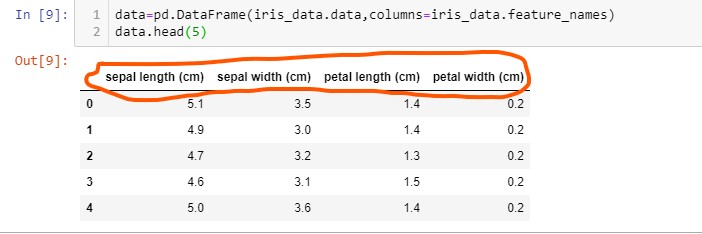
    In this dataset all the features (sepal length ,sepal width , petal length and petal width ) have real values. Feature count in a dataset can vary from 1 to 100K depending upon the problem to be solved. We use feature values to construct a Machine Learning model from them and also use these values directly or indirectly as input to that model for results.

  • Target or Labels:
  • In datasets each row of different feature values corresponds to some class or a real value which we want to predict or analyse, this coulmn in a dataset can be called as target or label column. Particularly in most of the ML the problem is to predict value or a class from the given value of features.

    The above code snippet displays 6 random rows, note that each row has 'class' specified under the 'target' column as one of the three values from setosa, versicolor or veginica. We can say that in this dataset target values has three classes, but in some other dataset target column can also have real vaulues.

  • Classification and Regression
  • Many times ML is used to solve predictive problems. The predictive problems can be classified into two categories:

    • Classification:
    • In these type of problems the target column contains the discrete values or different classes. For example it could either be divided into binary like 0/1 or may be into +ve and -ve class. Iris dataset is an example of classification problem in which we have class lables (setosa, versicolor and virginica). Some more examples of classification are:
      $(i)$ Predicting if the given review about some product is negative or positive- Target column may contain +ve and -ve or may be 0 for negative and 1 for positive.
      $(ii)$ Analysing the X-ray image of tumor and predicting if tumor is cancerous or not- Target column may contain 0 or 1 values.
      $(iii)$ Predicting if the given email can be categorized into spam or not- Target column may contain 0/1 or "spam"/"not spam" values

    • Regression:
    • In these type of predictive problems unlike classification, target column contains continous values. Most of the times in regression problems target values are real values.

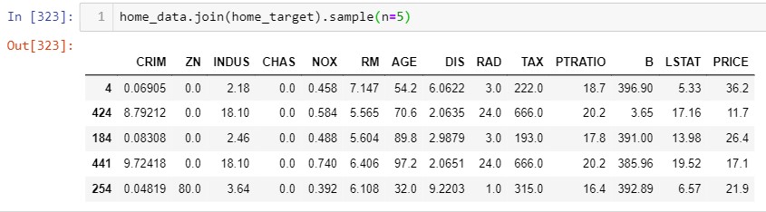
      The above snippet is from famous Boston house-price dataset, note that "Price" column being target column contains the prices of house based on the features from various aspects. In the target column we have real values as the median price of owner occupied homes in \$1000s. Some more examples of regression problems are:
      $(i)$ Predicting the price of a stock.
      $(ii)$ Predicting the release year of a song from audio features
      $(iii)$ Predicting the student performance in secondary education (high school).

  • Machine Learning Model:
  • A ML model can be described as any sequence of functions which take features as an Input and generates some prediction from them. For instance if we are given a task of predicting the class of iris flowers from a given set of 'features' then we need to make a model for this problem.
    Lets assume that we analysed the dataset and found the following inferences:
    $1.$ $99.5$% of flowers which have 'sepal length' below $5.6 cm$ are 'setosa'.
    $2.$ $93$% of flowers which have 'sepal width' less than $3.0 cm$ are either 'versicolor' or 'virginica'.
    Now as we have above inference, a simple ML model could be like :
    if sepal_length > 5.6:
      return 'versicolor or virginica'
    else:
     return 'setosa'

    The above code is just an intuition of ML model, in real world problems making an ML model is not that simple.

    As we know some basics of ML termiology we can start connecting dots between Mathematics and Data.

    K-NN - A perfect example of applied Mathematics

    K-NN (K Nearest Neighbours) is the simplest ML algorithm which is used for both classification and regression purposes. Understanding the internal working of K-NN algorithm will give us intituiton about how mathematics helps us to solve ML problems.

    Let us assume that we have a dataset with two features 'x' and 'y', both having real values and target column containing 0,1. Plotting the target column we can label them as Green and Red for 1 , 0 respectively on a 2D axis.
    Following table shows the structure of dataset:

    x y target
    1 x1 y1 0
    2
    x2
    y2
    1
    3 x3
    y3
    1
    4 x4
    y4
    0
    ... ... ... ...
    ... ... ... ...
    xytarget1x1y102...
    Viewer does not support full SVG 1.1

    Each data point can be represented as row vector for example data point $D_1$ can be represented as $\begin{bmatrix} x_1 & y_1\end{bmatrix}$
    Now a question that arises is, given a point $x_q$ with known features $\begin{bmatrix} x_q & y_q\end{bmatrix}$ is there any way we can classify it as 0 or 1 using the given data. Way the KNN algorithm works is based on the distace between the points or more formally as the difference between points. Just think if someone asks "Out of the list $[3,8,11,20,100,222]$ filter 3 numbers which are most closest to $2$ ", anyone can find that numbers by just taking difference between $2$ and each item in the list.
    This is the main idea behind the working of KNN, difference being in KNN we have to deal with the distance between vectors rather than scalers.
    To understand the algorithm completely, lets zoom into the above graphed points where the query point $x_q $ is located:

    In the above image if we calculate distance between $x_q$ and all the given points, the top 5 closest points to $x_q $ can be labelled. Now, out of top $5$ closest points to $x_q$ 3 are green and 2 are red i.e probabililty that $x_q$ belongs to Green (1) class is $\frac{3}{5}=0.6$ or there is $60\%$ chance that $x_q$ belongs to Green (1) class.

    Distance Calculation :

    As stated in part 1 the distance between two vectors is defined by the L-2 norm between two vectors. In this case distance between the query point $x_q$ and data points is:
    distance $=\sqrt{\sum_{i=1}^{m}(x_{qi}-d_i)^2}$
    where $m$ $\in$ number of features in a dataset.
    So if we want to find the similarity between $x_q$ and $d_1$=
    $\sqrt{(x_{q1}-x_1)^2+(y_{q2}-y_1)^2}$
    But we need to find the distance between all the points and $x_q$ to determine the top 5 closest distances. If total number of data points is $n$ then pseudo code to find the 5 shortest distance is :
    1.for each data point $d_i$ where i= 0 to n :
      measure L-2 norm between
    $x_q$ and $d_i$
      append the L-2 norm of $x_q$ and $d_i$ to list
    2.sort the list for first 5 shortest distances